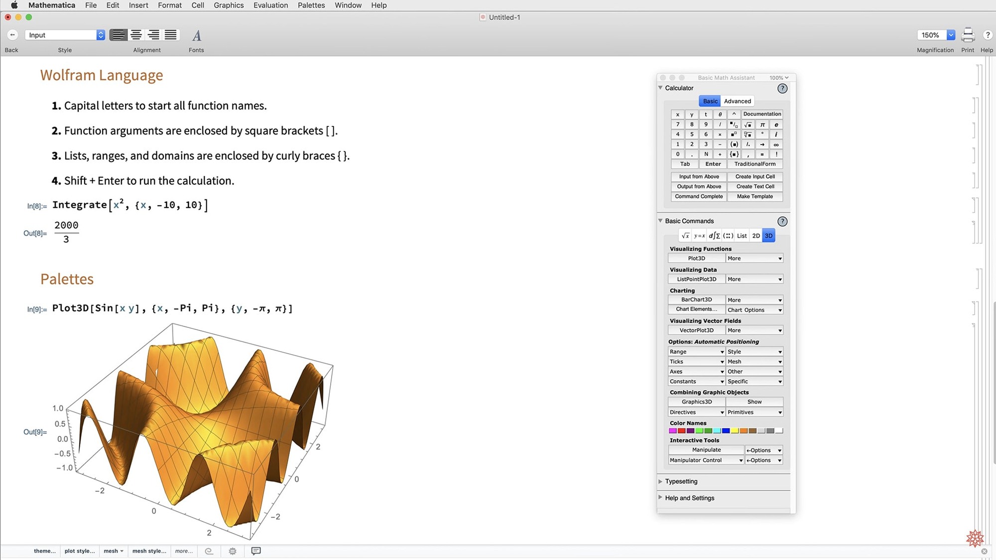
Wolfram Mathematica 15.0 — Mac build

Wolfram Mathematica 14.3.0 is the latest desktop release of Wolfram's technical computing environment. This version adds full dark mode support, new standard colors for both dark and light mode, and a range of new functions including Hilbert transforms, Lommel functions, geodesic computation, and LLMGraph. It also speeds up Python and R integration, adds ColumnwiseCombine, system model validation tools, and Markdown export. If you are looking to download a mathematica 12 download or a later version, here is what you need to know about running it on your Mac.

What version of macOS do I need?

Mathematica 14.3 runs on macOS 12 and later. That covers Monterey through the current release.

Supports both Apple Silicon and Intel Macs

It supports both. Apple Silicon (M1, M2, M3) and Intel 64-bit Macs are fully compatible.

Runs locally without an internet connection for core computation

One common question is whether Mathematica needs an active internet connection to run. The desktop application operates locally once installed. Cloud features like web browser access and external data imports require a connection, but the core symbolic and numerical computation, visualization, and notebook creation do not.

Another frequent topic is file compatibility between versions. Notebooks created in Mathematica 14.3 can generally be opened in earlier releases, though functions introduced in 14.3 — like LLMGraph or the new surface plotting tools — will not evaluate in older versions. The reverse is also true: notebooks from Mathematica 12 download or Mathematica 13 download open fine in 14.3, with no conversion step needed.

People also ask about using Mathematica alongside other tools. The 14.3 release specifically improved Python and R integration speed, so if you work across languages, that workflow has gotten faster. The Wolfram Language can call Python directly from notebooks, and R data can be pulled in and manipulated using Mathematica's symbolic engine.

Compares with MATLAB, Octave, and Maple for technical computing

Three applications overlap with Mathematica on macOS: MATLAB, GNU Octave, and Maple. Each serves a similar audience but takes a different approach.

MATLAB is strong on numerical computation and matrix operations. Its toolboxes cover engineering fields thoroughly, and Simulink adds model-based design. Mathematica counters with deeper symbolic capabilities — symbolic integration, differential equation solving, and formula manipulation that MATLAB handles less naturally. MATLAB's interface feels more procedural; Mathematica's notebook model lets you mix code, equations, and formatted output in one document. MATLAB runs natively on Apple Silicon. Mathematica does too.

GNU Octave is free and syntax-compatible with MATLAB. That is its main draw. It lacks Mathematica's symbolic engine, visualization breadth, and notebook interface. For quick numerical work Octave is fine. For symbolic math, data exploration with built-in functions, or producing publication-ready graphics, Mathematica has the edge. Octave's interface is basic. Mathematica's front end includes syntax highlighting, cell grouping, and the new dark mode in 14.3.

Maple is Mathematica's closest competitor in symbolic computation. Maple's clickable math interface is intuitive for equation entry, and its context menus let you perform operations without typing commands. Mathematica's natural-language input serves a similar purpose — type a sentence and it interprets the intent. Maple's visualization tools are solid but narrower than Mathematica's expanded 14.3 set, which now includes ListFitPlot, vector-based maps, and mesh processing. Maple runs on macOS but historically lags behind in Apple Silicon optimization.

Imported a CSV of temperature and stress values from a materials experiment

I opened Mathematica 14.3 to work through a data set from a materials experiment — temperature readings and stress values over time, stored in a CSV file. The first step was importing the data. I used Import with the file path, and Mathematica parsed the columns into a list of lists. The automatic type detection handled the numeric columns correctly on the first try.

I wanted to visualize the raw data before doing any modeling. The new ListFitPlot function in 14.3 was a natural choice: it plots data points and overlays a fitted curve in one call. I passed the imported list, specified a polynomial fit, and got a plot with the data points as markers and the fit as a solid line. The colors used the new standard palette for light mode, which looked clean on screen.

Next I ran a Hilbert transform on the stress signal to look for phase shifts. The Hilbert transform is new in 14.3, so I tried it expecting a function with the same syntax as other signal-processing commands. It returned a list of complex values representing the analytic signal. I plotted the real and imaginary parts on separate axes to confirm the shift. The whole chain — import, fit, transform, plot — ran in about a dozen lines.

I exported the final plots as Markdown for a project report. Markdown export is also new in 14.3. I selected the notebook cells, chose Export, and specified the Markdown format. The output preserved the code, the plots, and the text cells in a single .md file. No manual reformatting was needed.

Dark mode now covers the notebook interface, palettes, and dialog boxes

After installing, a few preferences make the environment more comfortable. If you work in low-light conditions, the dark mode toggle is under the Appearance settings. Version 14.3 applies it to the notebook interface, palettes, and dialog boxes consistently. The new standard colors adjust automatically between modes, but you can override individual style sheet colors if the defaults do not suit your data.

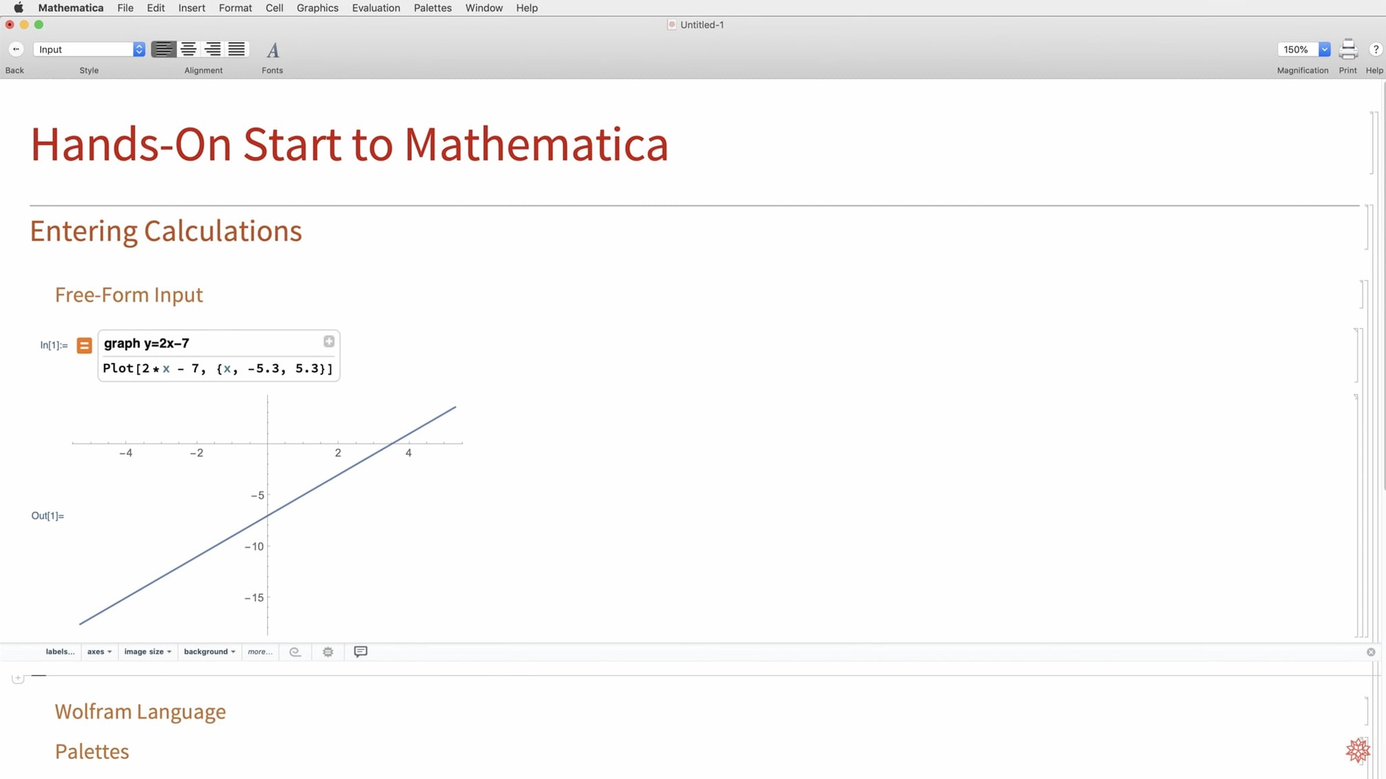
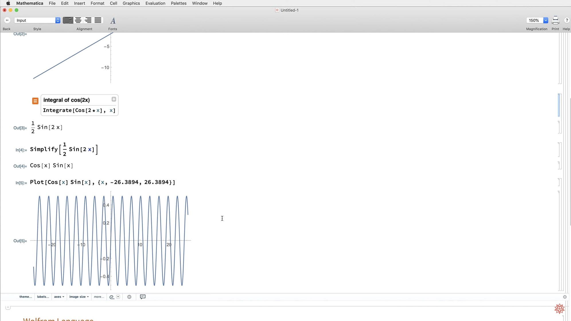
The natural-language input setting is worth enabling if you prefer typing queries in plain English. It lives in the Interface preferences. When active, typing "plot sin x from 0 to 2 pi" produces the same result as entering the formal Plot command. It saves lookup time for one-off calculations.

For those who work with external data regularly, setting the default import directory under File Locations reduces typing. Mathematica remembers the path, so subsequent Import calls can use relative paths or simple file names. It is a small change that saves time across a session.

The interface supports Russian, English, German, Vietnamese, Greek, Spanish, Italian, Chinese (Traditional and Simplified), Korean, Lithuanian, Polish, Portuguese, Ukrainian, French, and Japanese.

• Adds full support for dark mode.
• Introduces new standard colors for dark- and light-mode environments.
• Adds Hilbert transforms, Lommel functions, and new matrix decompositions.
• Expands visualization tools with ListFitPlot, surface plotting functions, vector-based maps, and mesh processing tools.
• Adds geodesic computation, LLMGraph, faster Python and R integration, ColumnwiseCombine, system model validation tools, and Markdown export support.

• macOS 12 or later
• Apple Silicon or Intel 64-bit Mac